4D imaging via remote refocus
This project is maintained by amsikking in the York lab, and was funded by Calico Life Sciences LLC
Appendix
Note that this is a limited PDF or print version; animated and interactive figures are disabled. For the full version of this article, please visit one of the following links: https://amsikking.github.io/remote_refocus https://andrewgyork.github.io/remote_refocus https://calico.github.io/remote_refocus
Remote refocus enables class-leading spatiotemporal resolution in 4D optical microscopy
Concept, rules and simulation
The idea
The basic concept of remote refocus is to make a 3D unity-magnification copy of the sample volume at a remote location, and then image this with a second microscope. Under normal operation, collecting light with a microscope objective away from the corrected focal plane will introduce aberrations that depend strongly on the effective de-focus and give unacceptably poor 3D image quality [Pawley 2006]. The 'magic' of RR is to use a standard microscope setup (objective/tube lens) in combination with a reversed copy of the optics (tube lens/objective) to produce an abberation-free 3D image - where the second microscope is configured to cancel the aberrations of the first. The detailed optical theory of RR is elegantly described in the original paper [Botcherby 2007] and will not be re-visited here. However, for those wishing to build an RR system, there are a few simple concepts and rules that should be highlighted.
Firstly there are two main optical arrangements (Figure A1) which we'll refer to as single objective remote refocus (SORR) and double objective remote refocus (DORR) for ease of discussion. DORR is the most straightforward implementation, and in its most elementary form consists of 3 identical microscopes back to back, where moving either the 2nd or 3rd objective will perform the refocusing. The simplest version of the SORR variant uses a single objective in a double pass configuration with an additional beam splitter optic and mirror. The re-focus in SORR is then performed by moving either the objective or the mirror.
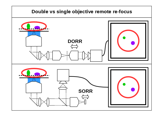
The main benefit of SORR is that the mirror can be very small and agile (<1 mm diameter) as it only has to cover the original sample scaled field of view (FOV), but the penalty is the introduction of the beam splitter optic. If a SORR is used with polarized light then the introduction of a quarter wave plate and polarizing beam splitter cube can give high optical efficiency. However in most imaging modalities light is unpolarized and so the splitter optic in the SORR arrangement results in an immediate signal loss of 50% with a polarizing splitter and quarter wave plate, or 75% with a 50/50 splitter. Despite this loss the SORR arrangement has been implemented in many microscopes due to the potentially high speeds and the relative simplicity of the optical train as discussed in the history section. However if maximum efficiency is prioritized then the DORR arrangement is preferable and inherently faster in 'photon limited' applications, and for this reason the DORR arrangement was pursued in this work.
The golden rules
Secondly there are a number of ‘golden rules’ for remote re-focus which must be respected to achieve best performance and are independent of the SORR or DORR arrangement.
- The magnification between the sample and its remote 3D copy should be set equal to the ratio of the index between these two locations: \[M_{RR} = \frac{n_{sample}}{n_{RR}}\] For an air based RR system with \(n_{RR}=1\) then this gives \(M_{RR}\approx1.5\) for oil and \(M_{RR}\approx1.33\) for water, etc.
- The optics downstream of the first objective should have enough clear aperture (CA) to accommodate the full wavefront as vignetting by any optic (tube lens or mirror etc.) will reduce resolution. It should be noted that the operation of RR expands the CA requirement beyond the normal range of a microscope, as defocused positions create non-infinity rays that may not be accommodated by the usual optical train. In this regard another critical consideration is that the RR objectives must have an angular acceptance that is greater than or equal to the first objective: \[\frac{\text{NA}_{RR}}{n_{RR}} \geq \frac{\text{NA}_{sample}}{n_{sample}}\] Again for an air based RR system with \(n_{RR}=1\) then this simplifies to: \[\text{NA}_{RR} \geq \frac{\text{NA}_{sample}}{n_{sample}}\]
- The individual objectives and tube lenses in the first two image relays which produce the 3D copy of the sample should approximate ideal lenses. RR theory is valid for lenses that well approximate ideal thin lenses placed in a 4f configuration, and deviating from this can have drastic effects on RR performance. It should be noted that not all objectives and tube lenses operate in this mode and so builders should choose their optics carefully. If you don't have detailed design information from your objective's manufacturer, we recommend you use the design we present here.
- The tube lenses between the first and second objective in the system should be in a telecentric 4f arrangement to give best performance. On a typical commercial microscope stand this is often not the case, as the distance between the objective and tubes lens can be less than one focal length for practical reasons. This does not affect performance during normal use, but can degrade RR operation.
How to check
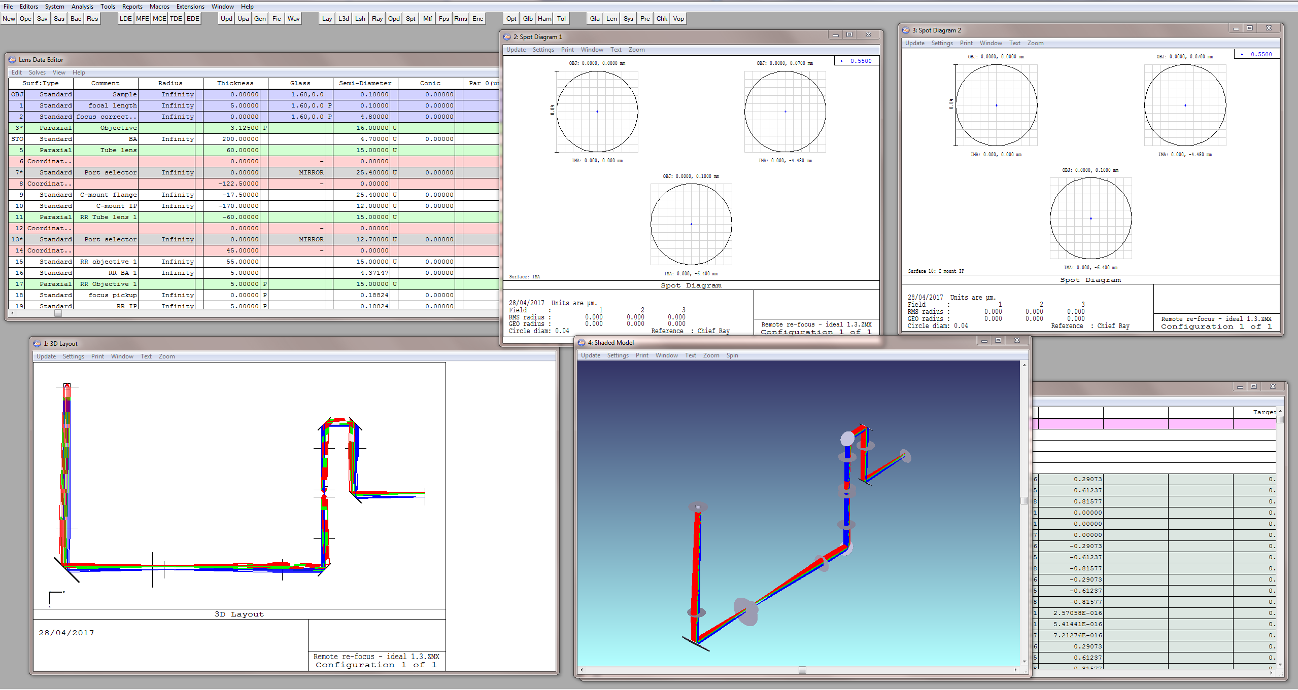
It should be noted that the aforementioned rules for remote refocus place substantial constraints on the optical design, and if followed carefully a well performing system can be built with relative ease, without the need for detailed optical design information or simulation. On the other hand, it can be difficult to know if a given objective is sufficiently "ideal". For those with access to detailed information about their optics and a suitable simulation software package like Zemax we recommend evaluating the performance of a possible RR configuration before building (Figure A2). Even for a novice designer this process can be relatively straightforward with the following workflow:
- Start by laying out a simple DORR optical train with ideal elements that match the diameters and focal lengths of the intended build and adhere to the ‘golden rules’ of RR.
- Defocus the sample and chase the image with one of the RR objectives by the magnification factor between the conjugate planes (1st golden rule). The RR should work perfectly and any basic mistakes in design will be highlighted at this point and can be easily corrected.
- Now substitute in real components and evaluate the performance of the RR over its axial range. All of the non-idealities of the system will now show to give a finite range over which the real system can be expected to be diffraction limited (DL) if built and aligned correctly.
Design
A high performance remote refocus for a 60x oil objective
In this section a recipe for a high performance remote refocus in the DORR configuration is given and presented as a versatile addition to a typical microscope stand. This RR module is designed to work with a high NA 60x oil immersion objective and is capable of producing multicolor DL stacks over the full FOV of a standard sCMOS camera. The emphasis in this design was on achieving a high performance RR using minimal custom parts. In this vein, all of the optics and the majority of the mechanics are relatively low cost, short lead time stock parts, with only a few simple bespoke mechanics where needed. The merits and choices of the design will now be discussed in turn and the reader may refer to the build section for a full list of parts, drawings and an alignment procedure.
To avoid custom optics, this DORR is based on the readily available Nikon 60x 1.4 NA oil and 40x 0.95 NA air objectives that, together with stock tube lenses, very conveniently obey the first three golden rules of RR, with the 4th rule achieved by setting the right mechanical spacing of the elements (see drawings). By working closely with Nikon, we were able to establish excellent performance with a 450-650 nm polychromatic Strehl ratio >0.74 over an axial range of +/-32 μm in the sample with a 150 μm diameter field of view.
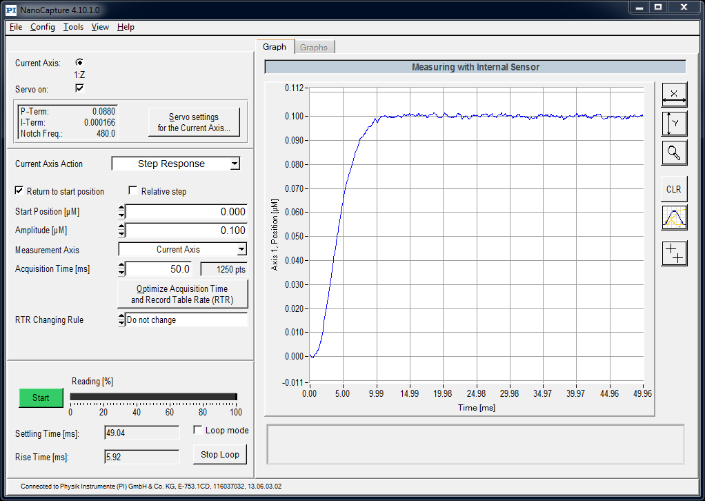
With good optical design established, the choice of Z-drive actuator was made relatively straightforward - an axial range of +/-32 μm in the sample with an index of ~1.5 corresponds to motion in air of ~+/-50 μm, which sits comfortably in the range of high performance piezo actuators - like the heavy duty PI 726 that can move a ~200 g objective at >500 Hz over a 100 μm range. The 726 can achieve step-and-settle times in the 0.1-1 μm range in <10 ms (Figure A3), which is faster than the rolling time of a good sCMOS camera like the PCO.edge 4.2 at full field of view. This equates to a running mode of 100 fps, giving 10 volumes per second for a 10-slice stack.
Piezo (step size)
Cropping the camera chip can produce higher frame rates for the fastest acquisitions, but in this regime the rolling time of the camera can be shorter than the step-and-settle time of the piezo, and motionless frames are no longer straightforward. It is straightforward, however, to operate the piezo in a constant-velocity mode, by sending a triangle wave signal to its analog input with an amplitude that corresponds to the desired stack size. The camera can then take frames at a high rate as the piezo moves continuously through the sample to give fast volumetric imaging but with an extended depth of field. It should also be noted that due to current limitations on sCMOS cameras the increased frame rates are achieved by cropping only one axis (up/down) with no benefit to cropping the second axis (left/right), and this forces elongated fields of view that may not be appropriate for all samples.
This motion solution prioritizes performance above economy, but may be substituted for other devices for those on a budget. Z-drive flexibility is a second-order advantage of using the RR arrangement - large, atypical actuators that would otherwise be awkward to fit to a typical microscope can be accomodated with relative ease and do not interfere with normal operation of the stand.
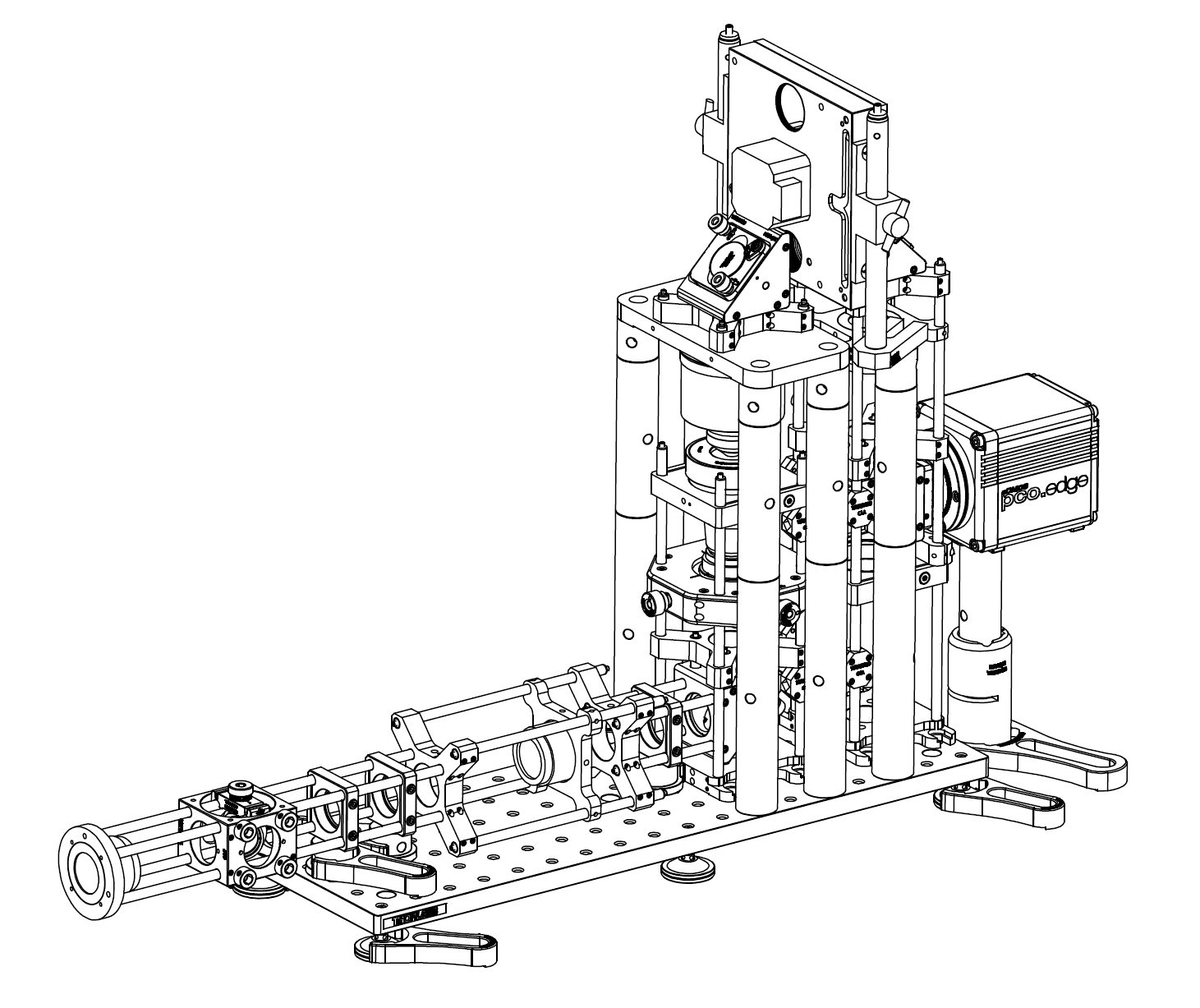
The RR optics are folded with 4 standard 1" highly reflective mirrors, both to give a more compact footprint and also orientate the RR objectives into the vertical position for mechanical stability. The mirrors are housed in standard 3-axis kinematic mounts for ease of alignment and were noted to be slightly undersized at the design phase. This causes a small amount of vignetting in the corners of the sCMOS FOV at diameters >17.5 mm, but seemed like a good trade rather than upgrading to 2" mirrors and substantially increasing the size and cost of the module for relatively little gain. The fold arrangement accommodates common incubation chambers by keeping the optical train low and long out of the microscope side port, which is desirable for many live cell applications.
Another critical part of the design is the ability to align and stabilize the RR objectives, as unwanted motion here will translate directly into the image, making it the most sensitive part of the module. The Z-drive piezo/objective assembly is therefore mounted on a heavy-duty frame and isolated from the adjustable objective, which is mounted on an X/Y/Z translation stage to give the fine adjustment needed for alignment. Both RR objectives benefit from the gravitationally-aligned, axially symmetric vertical arrangement, which avoids many of the unwanted drifts and motions that can occur in alternative setups. Stability testing showed X/Y drifts in the 150 nm/hour range for the combined sample, stage, microscope and RR which seems acceptable given typical lab thermal drift and the intended sub-minute run time of a typical acquisition. All of the standard short lead-time optomechanics were sourced from Thorlabs and could be substituted for equivalent parts from existing lab stock.

An AR-coated 1" 340 μm coverslip correction glass window was ordered from Mark Optics and inserted between the two 40x air objectives to give best performance, as they are optimised to work with 170 μm of glass. An estimate for the optical efficiency of the RR was then calculated at ~70% with (0.92)(0.952)(0.994)(0.99) for the objectives, tube lenses, mirrors and glass window respectively and was subsequently measured at >73% (Figure A6). For those looking to save on cost, the glass window can also be composed of two standard coverslips sandwiched together with some immersion oil, with the penalty of ~5% loss in signal.


A flexible slot was reserved in the infinity space behind the last objective for the inclusion of a high speed emission filter wheel like the ASI FW-1000, which we chose for its high speed trigger options and <40 ms switching time. This can be mounted on the RR breadboard or directly to the optical table to avoid any unwanted vibrations that can couple from the torque generated by fast wheels. Of course, any filter wheel that physically fits can be used here - including a low-cost manual wheel from Thorlabs that will connect directly to the mechanics for starting off. The camera is easily focused by sliding the Z-position of the last mirror and orientated correctly with the built-in rotation mount, and the caged mirror on the input arm can be used to pull out the intermediate image plane without removing the instrument, if needed. The remaining custom parts were prepared by Zera Development, but can be also readily milled by almost any CNC machine shop; see the drawings section for details. If you're unfamiliar with machine shops, simply send a copy of the drawing we provide to Zera.
Build
List of parts
This table can be used as a shopping list for the RR described in this article. Item 37 is a low cost manual filter wheel that can be substituted for an automated wheel if needed, and item 49 can be avoided to reduce cost (substite with two coverslips sandwiched together with oil). With some re-design work, items 38-40 can be substituted for a lower cost option although this is not encouraged as it may negate the intended high speed operation of the device.
| Item No. | Supplier | Part | Description | Qty |
|---|---|---|---|---|
| 1 | Thorlabs | MB1545/M | Aluminum Breadboard, 150 mm x 450 mm x 12.7 mm, M6 Taps | 1 |
| 2 | Thorlabs | SWB/M | Articulated Mounting Base, M6 x 1.0 Threaded Stud, Qty. 1 | 6 |
| 3 | Thorlabs | ER10 | Cage Assembly Rod, 10" (254.0 mm) Long, Ø6 mm | 4 |
| 4 | Thorlabs | C6W | 30 mm Cage Cube, Ø6 mm Through Holes | 1 |
| 5 | Thorlabs | CP08/M | SM1 Threaded 30 mm Enhanced Clamping Cage Plate, 0.35" Thick, M4 Tap | 3 |
| 6 | Thorlabs | RS075P4M | Ø25.0 mm Pedestal Pillar Post, M4 Taps, L = 19 mm | 3 |
| 7 | Thorlabs | CF125 | Short Clamping Fork, 1.24" Counterbored Slot, Universal | 7 |
| 8 | Thorlabs | LCP02/M | 30 mm to 60 mm Cage Plate Adapter, M4 Tap | 6 |
| 9 | Thorlabs | ER6 | Cage Assembly Rod, 6" (152.4 mm) Long, Ø6 mm | 4 |
| 10 | Thorlabs | ER3 | Cage Assembly Rod, 3" (76.2 mm) Long, Ø6 mm | 4 |
| 11 | Thorlabs | ERSCA | Rod Adapter for Ø6 mm ER Rods, Qty. 1 | 4 |
| 12 | Thorlabs | CP360R/M | Pivoting, Quick-Release, Ø1" Optic Mount for 30 mm Cage System (Metric) | 1 |
| 13 | Thorlabs | BB1-E02 | Ø1" Broadband Dielectric Mirror, 400 - 750 nm | 5 |
| 14 | Thorlabs | CPVM | Vertical Cage System Mounting Plate | 2 |
| 15 | Thorlabs | ER8 | Cage Assembly Rod, 8" (203.2 mm) Long, Ø6 mm | 4 |
| 16 | Thorlabs | KCB1C/M | Right-Angle Kinematic Mirror Mount with Smooth Cage Rod Bores, 30 mm Cage System and SM1 Compatible, M4 and M6 Mounting Holes | 4 |
| 17 | Thorlabs | ER1 | Cage Assembly Rod, 1" (25.4 mm) Long, Ø6 mm | 20 |
| 18 | Thorlabs | CXYZ1/M | XYZ Translation Mount for Ø1" Optics, M6 Taps | 1 |
| 19 | Thorlabs | SM1A12 | Adapter with External SM1 Threads and Internal M25 x 0.75 Threads | 1 |
| 20 | Thorlabs | LCP08/M | 60 mm Cage Plate, SM2 Threaded, Enhanced Clamping, 0.5" Thick, M4 Tap (One SM2RR Retaining Ring Included) | 2 |
| 21 | Thorlabs | SM2V05 | Ø2" Adjustable Lens Tube, 0.31" Travel | 1 |
| 22 | Thorlabs | SM2A6 | Adapter with External SM2 Threads and Internal SM1 Threads | 1 |
| 23 | Thorlabs | RS150/M | Ø25 mm Post, L = 150 mm | 6 |
| 24 | Thorlabs | RS100/M | Ø25 mm Post, L = 100 mm | 6 |
| 25 | Thorlabs | RS25/M | Ø25 mm Post, L = 25 mm | 6 |
| 26 | Thorlabs | ER05 | Cage Assembly Rod, 1/2" (12.7 mm) Long, Ø6 mm | 12 |
| 27 | Thorlabs | ER12 | Cage Assembly Rod, 12" (304.8 mm) Long, Ø6 mm | 4 |
| 28 | Thorlabs | LCP01B | 60 mm Cage Mounting Bracket | 1 |
| 29 | Thorlabs | SM1A39 | Adapter with External C-Mount Threads and External SM1 Threads | 1 |
| 30 | Thorlabs | CRM1/M | Cage Rotation Mount for Ø1" Optics, SM1 Threaded, M4 Tap | 1 |
| 31 | Thorlabs | RS100/M | Ø25 mm Post, L = 100 mm | 1 |
| 32 | Thorlabs | RSH3/M | Ø25 mm Post Holder with Flexure Lock, Pedestal Base, L = 75 mm | 1 |
| 33 | Thorlabs | PF175 | Clamping Fork for Ø1.5" Pedestal Post or Post Pedestal Base Adapter, Universal | 1 |
| 34 | Thorlabs | C1A | ER Rod Cross Coupler, Top and Bottom Pieces | 8 |
| 35 | Thorlabs | BA1S/M | Mounting Base, 25 mm x 58 mm x 10 mm | 2 |
| 36 | Thorlabs | TR150/M | Ø12.7 mm Optical Post, SS, M4 Setscrew, M6 Tap, L = 150 mm | 2 |
| 37 | Thorlabs | CFW6 | 30 mm Cage Filter Wheel for Six Ø1" Filters | 1 |
| 38 | PI | P-726.1CD | PIFOC® Ultra-High-Dynamics Microscope Lens Piezo-Z Positioning Drive, 100μm travel | 1 |
| 49 | PI | P-726.11 | P-726 PIFOC® Thread Adapter M25 | 1 |
| 40 | PI | E-753.1CD | High-Speed Single-Channel Digital Piezo Controller for Capacitive Sensors | 1 |
| 41 | Nikon | MXA22018 | Tube lens 200mm EFL | 3 |
| 42 | Nikon | MRD00405 | CFI Plan Apo Lambda 40x - 0.95NA, WD0.25-0.16 | 2 |
| 43 | Nikon | MRD01605 | CFI60 Plan Apochromat Lambda 60x Oil Immersion Objective Lens, N.A. 1.4, W.D., 0.13mm, F.O.V. 25mm, DIC | 1 |
| 44 | Zera Development | DMi8 casting flange adaptor 1.0 | Adaptor for connecting a 6x30mm cage system to the cast flange of the DMi8 camera side port. This version is for the right hand port (left hand version requires M3 holes mirrored on optical axis). | 1 |
| 45 | Zera Development | Objective holder plate M25x0.75 | Adaptor plate for integrating M25 x 0.75 objectives into a 6x60mm cage system with M6 counter sunk holes for metric breadboards. Exact thickness is design specific. | 1 |
| 46 | Zera Development | Tube lens adaptor M38 x 0.5 for 60mm cage 1.0 | Adaptor plate for including M38 x 0.5 threaded parts into a 60mm cage system on axis. | 2 |
| 47 | Mark Optics | Custom | Custom glass window: Window, Coated, Bk-7, OD: 25mm +/- 0.2mm, Thk: 0.34mm +/- 0.1mm, polished both sides 20/10, TWF 1/4 wave, parallelism < 10 arc sec, CA 90%, VIS AR coated Tavg >99% 400-700nm, AOI = 0 degree | 1 |
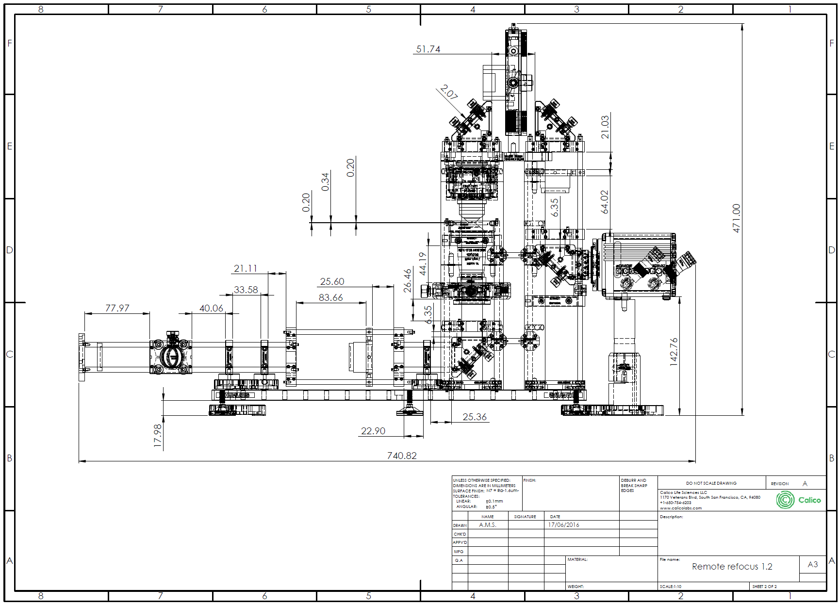
Drawings
For 2D CAD drawings please refer to this folder, and for full-sized assembly drawings, please click here. For our custom parts, .STEP files can be found here and 3D CAD for all other parts can be sourced from the respective manufacturers.
Alignment procedure
Aligning the RR for someone with optical assembly and microscopy experience is straightforward. For those unsure as to how to proceed, please try one of the following alignment procedures, bearing in mind that alignment is iterative and usually a learning process. The first time might take a day or two, the Nth time less than an hour...
- Alignment with extended tool set and full access to components:
- Collimate a small diameter (<1 mm) low power (<1 mW) laser beam over a few meters and axially align the beam with the appropriate microscope thread (usually M25x0.75 or RMS).
- Remove all the lenses from the system (three objective/tube lens pairs) and the camera.
- Fire the laser beam through the microscope from the primary objective thread and out through the side port and through the RR optical train.
- Use pinholes or irises to firstly align the RR to the microscope by adjusting the height of the feet and the relative position on the table (then bolt down).
- Now use pinholes or irises to axially align the rest of the path using the RR tip tilt mirrors. At the end of this step the beam should be centered in X/Y at every point in the system from the primary objective to the camera.
- Now remove the laser, add the camera and fit the lenses as close as possible to their designed positions ready for imaging.
- Image a known sample (like a graticule) with transmitted light and focus with the eye pieces. Now image with the RR camera and (with the piezo powered and in its nominal rest position) use the X/Y/Z mount on the adjustable objective to focus and center the sample.
- Now de-focus with the microscope stand and re-focus with the RR to check function. Minor adjustments to the mirrors and X/Y/Z objective may be needed for good alignment.
- Alignment with limited tools and access
- Image a known transmitted light sample (like a graticule) with the primary objective tube lens pair on the microscope using the eyepieces to centre and focus.
- Remove the RR lenses (two objective tube lens pairs) and the camera.
- Set the white light source to maximum intensity and darken the room so that the beam is visible throughout the system.
- Use pinholes or irises to firstly align the RR to the microscope by adjusting the height of the feet and the relative position on the table (then bolt down). A graticule with a well-chosen scale can have a visible image (crosshairs) that can be used at the magnified image plane to get good alignment.
- Now use pinholes or irises to axially align the rest of the path using the RR tip/tilt mirrors. At the end of this step the beam should be centered in X/Y at every point in the system, from the primary objective to the camera.
- Add the camera to the RR and fit the lenses as close as possible to their designed positions ready for imaging.
- Image with the RR camera and (with the piezo powered and in its nominal rest position) use the X/Y/Z mount on the adjustable objective to focus and center the sample.
- Now de-focus with the microscope stand and refocus with the RR to check function.
- Adjustments to the position of the RR base, mirrors and X/Y/Z objective will likely be needed for good alignment - expect to iterate.
Acquisition
Additional equipment
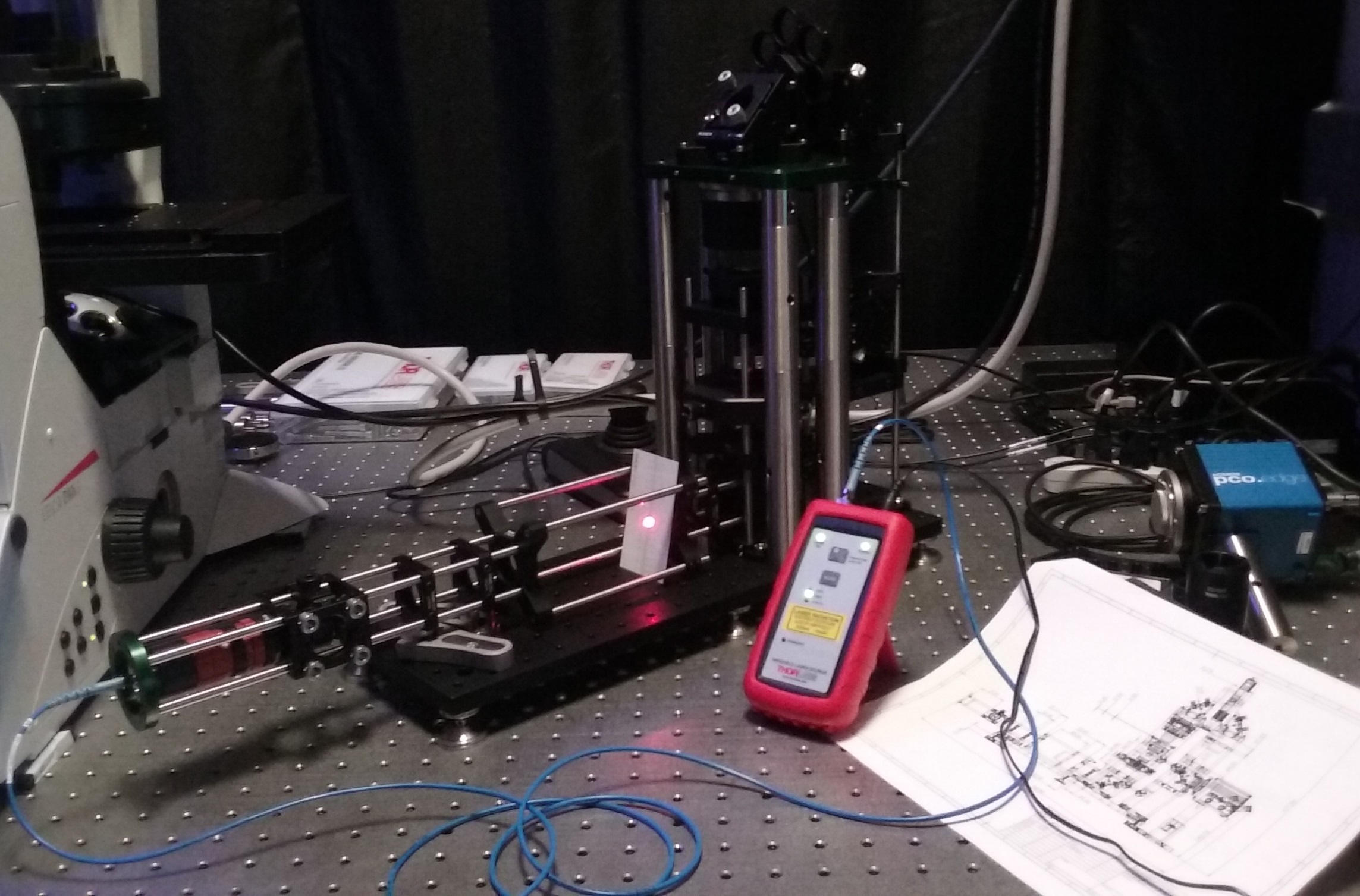
To evaluate the RR we used the following additional equipment in our experimental setup
| Item No. | Supplier | Part | Description |
|---|---|---|---|
| 1 | Leica | DMi8 | Research-grade inverted microscope stand with motorized Z-drive |
| 2 | PI | U-780 | Automated XY stage, 100 nm precision, closed-loop PID control |
| 3 | PI | P-737 | Z-piezo stage insert, 500 μm travel, 100 Hz resonant fequency (200 g load), closed loop PID control with 5 kHz analog-in |
| 4 | Lumencor | SpectraX | Multicolor LED light source with TTL trigger (10 μs rise/fall) |
| 5 | PCO | edge 4.2 | sCMOS camera, 2048x2048 pixels with 6.5x6.5 μm2 size, 100 fps full field, TTL trigger <50 μs response |
| 6 | NI | PCI-6733 | 8 channel analog-out card, 1 MHz, 16 bit |
| 7 | Zera Development | DMi8 stage spacer 15mm front 1.0 | Raises XY stage on DMi8 platform by 15 mm to accomodate objectives with longer parfocal distance or piezo Z-drive inserts that require more height. |
| 8 | Zera Development | DMi8 stage spacer 15 mm rear 1.0 | Raises XY stage on DMi8 platform by 15 mm to accomodate objectives with longer parfocal distance or piezo Z-drive inserts that require more height. |
| 9 | Thorlabs | PL15M25 | 15 mm Parfocal Length Extender for Microscope Objectives, M25 x 0.75 Threading |
How we took our data
With the above mentioned hardware setup we used Python scripts to issue serial port commands to devices and create voltages to play with the National Instruments analog-out card. In practice, data was taken by focusing on the sample with the microscope Z-drive to give the ‘zero’ or reference position. Focus was then adjusted by using either the microscope Z, the piezo Z stage insert, or the remote refocus piezo depending on the mode of operation.
The original data presented in this article is available to download from Zenodo (17.5 GB, DOI: 10.5281/zenodo.1145453) and can be unziped (27.3 GB) and used with the figure generation code to reproduce the figures in the main text.
Example code
Here we annotate a typical example of the script that was used for data collection. The exact script for each data set was not kept, as it amounted only to minor changes in stack amplitude, step size, exposure, etc., or changes in the order of operation or routine depending on the experiment. Base examples of the scripts used for biological imaging and motion performance can be found in the data generation folder, including the associated dependencies for running the hardware, with the exception of the microscope stand the control of which cannot be made public due to a proprietary API.
- Necessary python modules are imported, followed by hardware control scripts. The program then checks if it's the 'main' program and if so imports the multiprocessing module needed for image_data_pipeline.py which runs the camera. A sensible level of verbosity is then set using the logger commands.
# Built-in Python modules import time import tkinter # Third party, but highly standard Python module import numpy as np # Custom scripts we've written for hardware control # See: https://github.com/AndrewGYork/tools import ni import leica_scope import physik_instrumente import image_data_pipeline import lumencor from pco import pco_edge_camera_child_process, legalize_roi if __name__ == '__main__': import multiprocessing as mp import logging logger = mp.log_to_stderr() logger.setLevel(logging.INFO) - COM ports are assigned to the hardware with serial control, and analog-out channels are given to the camera, RR and light source:
### COM port assignment dmi8_com_port = 'COM4' rr_piezo_com_port = 'COM6' epi_com_port = 'COM10' ### Analog out channel settings ao_ch = {'camera' :0, 'rr_piezo' :1, 'spx_uv' :2, 'spx_blue' :3, 'spx_cyan' :4, 'spx_teal' :5, 'spx_green' :6, 'spx_red' :7,} ao_ch_name = {} for name, index in ao_ch.items(): ao_ch_name[index]= name - The user sets the choice of objective to be either the 40x 0.95 NA air or 60x 1.4 NA oil. The RR instrument was designed to work with both objectives, but the 'z_ratio' which is the amount the RR piezo needs to move in air to give a certain de-focus in the sample, changes according to the 1st golden rule of RR. In practice with the optics used, we found 0.98 to be correct for air and 1.42 for oil when imaging the Argolight slide. This was calibrated by de-focusing a known amount with the microscope and then seeing what piezo offset was needed to refocus.
### Objective choice objective = 'oil' # Choose 'air' or 'oil' # 'air':0.98 for best correction collar setting of 0.19 for Argolight # 'oil':1.42 z_ratio = {'air':0.98, 'oil':1.42}[objective] - Acquisition parameters are chosen including stack amplitude, step size, number of colors, number of volumes to image, exposure time and file name format. Sensible bounds of memory buffer size and camera chip region-of-interest are asserted to avoid crashes.
### Stack parameters stk_amp = 5 # set half amplitude of stack around current focus (um) stk_step_size = 1 # set stack step size (um) stk_num_steps = round(2 * stk_amp / stk_step_size) + 1 # RR stack conversion rr_stk_amp = stk_amp * z_ratio ### Volumetric image information num_vol = 2 num_colors = 2 # To change from 2 must edit voltage code num_frames = stk_num_steps * num_vol * num_colors assert num_frames < 1001 # Set sensible upper bound on buffer ### Illumination settings tl_ao_ch = ao_ch['spx_green'] # take an epi channels for trans light led_ao_ch = ao_ch['spx_cyan'] # set epi excitation color led_intensities = {'uv':255, # set epi excitation intensities 'blue':255, 'cyan':255, 'teal':255, 'green':255, 'red':255,} ### Camera settings exposure_ms = 20 # set exposure - includes rolling time (ms) filename_format = '%s_%s_vol_%sum_stk_%sum_step_%sms_exp.tif' # (led_ao_ch, num_vol, stk_amp, stk_step_size, exp_ms) roi = legalize_roi({'top':1, # Be careful to choose a 'legal' roi! ## 'left':1, ## 'right':2060 }) - The camera, analog-out card, microscope, LED light source and RR piezo are initialized. The camera is controlled through the
image_data_pipeline.pymodule which simultaneously handles grabbing frames, displaying to screen and saving to disk using multiprocessing. The data rate for the analog-out card is set at least 10x higher than the fastest acquisition event to ensure synchronization, and the microscope tube lens turret is moved to an empty position so as to not obscure the remote refocus optics. The RR piezo is centered on its reference position and a 'position to voltage' function is defined for analog control:### Initialize hardware # Camera idp = image_data_pipeline.Image_Data_Pipeline( num_buffers=1, buffer_shape=(num_frames, # Buffer size for full volume series roi['bottom']-roi['top']+1, roi['right']-roi['left']+1), camera_child_process=pco_edge_camera_child_process) idp.apply_camera_settings( exposure_time_microseconds=exposure_ms*1000, trigger='external_trigger', preframes=0, region_of_interest=roi) ao = ni.Analog_Out( num_channels='all', rate=1e5, # Voltages per second daq_type='6733', board_name='Dev1') # Microscope dmi8 = leica_scope.DMI_8_Microscope(dmi8_com_port) dmi8.set_max_pos_magn(max_n=4) dmi8.change_magn(4) # Set tube lens to empty position # Epi light source epi_source = lumencor.SpectraX(epi_com_port, verbose=False) epi_source.set_intensity(**led_intensities) # Remote re-focus piezo rr_piezo = physik_instrumente.E753_Z_Piezo(which_port=rr_piezo_com_port, verbose=False) rr_piezo.move(50) # Send piezo to default zero position (um) rr_piezo._finish_moving() rr_piezo.set_analog_control_state(True) def piezo_volts_from_pos(desired_piezo_offset_um): piezo_position_abs = 50 + desired_piezo_offset_um piezo_analog_in_voltage = (piezo_position_abs - 50) / 5 assert -10 <= piezo_analog_in_voltage <= 10 return piezo_analog_in_voltage - A voltages vs. time array is created for each channel of the analog-out card for device control (the default is zero volts for channels that are not specified). The exposure time set in the acquisition section is split into camera rolling time (time needed for camera to initialize all pixels) and actual exposure time (time when the LED can be on and data can be taken) with an additional 'jitter time' added to ensure the camera doesn't miss the next trigger after an exposure. With the timeline established, 'lights on' time windows and piezo movements can be given according to the acquisition parameters.
### Set up voltages for analog out control # Camera timing information TTL_HIGH_V = 3 # 3V TTL rolling_time_s = idp.camera.get_setting('rolling_time_microseconds')*1e-6 exposure_time_s = idp.camera.get_setting('exposure_time_microseconds')*1e-6 jitter_time_s = 50e-6 assert rolling_time_s < exposure_time_s jitter_pix = round(jitter_time_s * ao.rate) assert jitter_pix > 1 # Helps ensure the camera won't swallow a trigger start_pix = jitter_pix + round(rolling_time_s * ao.rate) stop_pix = round(exposure_time_s * ao.rate) # Create voltage list and voltage shape voltages_list = [] # To fill with numpy arrays voltage_shape = (stop_pix + jitter_pix, ao.num_channels) # Create voltages for volumes for v in range(num_vol): # Create voltages for stacks for rr_piezo_z in np.linspace(-rr_stk_amp, rr_stk_amp, stk_num_steps): # Create voltages for frames # Transmitted light tl_frame_voltages = np.zeros(voltage_shape, dtype=np.float64) tl_frame_voltages[:start_pix, ao_ch['camera']] = TTL_HIGH_V tl_frame_voltages[start_pix:stop_pix, tl_ao_ch] = TTL_HIGH_V tl_frame_voltages[:, ao_ch['rr_piezo']] = piezo_volts_from_pos( rr_piezo_z) voltages_list.append(tl_frame_voltages) # Epi led excitation led_frame_voltages = np.zeros(voltage_shape, dtype=np.float64) led_frame_voltages[:start_pix, ao_ch['camera']] = TTL_HIGH_V led_frame_voltages[start_pix:stop_pix, led_ao_ch] = TTL_HIGH_V led_frame_voltages[:, ao_ch['rr_piezo']] = piezo_volts_from_pos( rr_piezo_z) voltages_list.append(led_frame_voltages) rr_stk_amp = -rr_stk_amp # bidirectional z scanning for speed # Combine voltages into single array voltages = np.concatenate(voltages_list, axis=0) - This optional code is useful for capturing live biological events that are seen on-screen in a preview mode. The user can watch the sample in real time, and hit the acquire button when something interesting happens. The script turns on the light source and continuosly runs the camera in a loop (displaying to screen), until the user closes the window at which point the acquisition begins immediately.
### Prepare and run livemode for preview of sample # Turn on transmitted light tl_on_voltage_shape = (10, ao.num_channels) # 10 time units wide tl_ao_ch_high = np.zeros(tl_on_voltage_shape, dtype=np.float64) tl_ao_ch_high[:, tl_ao_ch] = TTL_HIGH_V ao.play_voltages(tl_ao_ch_high, force_final_zeros=False) # Reset camera buffer for livemode idp.apply_camera_settings(frames_per_buffer=1) # For livemode image def live_mode(): # Tell the camera to start trying to take an image idp.load_permission_slips(num_slips=1) idp.camera.commands.send(('force_trigger', {})) assert idp.camera.commands.recv() # Trigger must be successful # Wait for any previous image to finish: while len(idp.idle_data_buffers) == 0: idp.collect_permission_slips() tk.after(1, live_mode) # Re-schedule livemode # Set up event loop for livemode tk = tkinter.Tk() tkinter.Label(tk, text="Close window to take a volumetric series").pack() ## tkinter.Button(tk, text="Snap", command=live_mode).pack() tk.after(1, live_mode) # Schedule 1st instance of live mode in event loop tk.mainloop() # Run event loop for livemode - The camera is reset after the preview mode, and the analog-out card now plays the pre-defined voltage arrays to run the acquisition and save files to disk.
### Reset camera properties for ao triggered stack idp.apply_camera_settings(frames_per_buffer=num_frames) # Reset for volumes # Wait for any previous file saving to finish: while len(idp.idle_data_buffers) == 0: idp.collect_permission_slips() # Tell the camera to start trying to take stacks and where to save idp.load_permission_slips( num_slips=1, file_saving_info=[ {'filename': filename_format %(ao_ch_name[led_ao_ch], num_vol, 2*stk_amp, stk_step_size, exposure_ms)}]) while not idp.camera.input_queue.empty(): # Is the camera ready? pass # If not then hold ao play until camera is ready ### Play analog voltages start = time.perf_counter() ao.play_voltages(voltages) end = time.perf_counter() ## print('Time elapsed in seconds =', end - start) ## input('hit enter to continue...') - Hardware elements are released, ready for the next acquisition:
    ### Close all objects
    idp.close()
    ao.close()
    dmi8.close()
    rr_piezo.close()
History
A summary of RR publications
Since the original RR paper [Botcherby 2007], there have been many publications that have used this technique for a variety of applications. The aim of this section is provide a very concise summary of these developments, to help the reader frame the use of RR within the field of microscopy.
[Botcherby 2008] applied a SORR to a spinning disk confocal microscope operating in an extended depth of field (EDF) mode to give Z-projections onto a single camera exposure. This had the advantage of achieving high frame rates due to a small scanning mirror, at the expense of ~50% of the fluorescence light, which is currently the main drawback of the SORR arrangement. A tilt mirror close to the back focal plane (BFP) was added to give angular variations of the EDF image over a small range giving an effective 3D perspective of the sample. [Dunsby 2008] modified the DORR concept to invent the oblique plane microscopy (OPM) modality, which enables light-sheet illumination and collection from a single high-NA objective. This breakthrough resulted in a true ‘single objective’ light sheet microscope, removing the many drawbacks of multi-objective systems but with the inherent limitation of lower effective resolution and collection efficiency due to the tilted arrangement of the optics. For oil immersion objectives, this equates to a maximum effective numerical aperture of about 1, with a ~50% loss in fluorescence signal.
[Botcherby 2009] used SORR in combination with a line-illumination and slit confocal microscope arrangement, including a secondary scanning mirror, to pack lines onto the camera and produce high frame rates in the meridional or Z-plane of the sample. This SORR setup had the usual drawback of ~50% signal loss due to the polarizing beam splitter (PBS) cube, but was a nice early demonstration of how RR can be appended to an existing imaging platform. [Salter 2009] demonstrated the use of SORR in a two-photon microscope for analysing liquid crystal dynamics in Z.
[Hoover 2011] used SORR with their differential multiphoton microscopy technique to give agile Z-adjustment, and [Kumar 2011] improved on the original OPM setup by coupling the excitation through the RR so that the light sheet and image plane can be simultaneously swept through the sample in a remote fashion to give inherently synchronized imaging at high volumetric frame rates. [Anselmi 2011] combined SORR with 3D holographic stimulation and introduced a novel tilt of the RR scan mirror that is similar in concept to the OPM setup, and allows imaging of tunable oblique planes in the sample. The paper also offers a thorough quantification of RR performance with the optics used in the experiment confirming the analysis of the original paper [Botcherby 2007]. [Smith 2011] combine SORR with a traditional point-scanning two-photon microscope to give agile axial adjustment and the ability to create oblique excitation planes via high speed synchronized 3D point scanning.
[Botcherby 2012] optimise their SORR for a two-photon microscope for high acquisition rates and present relevant applications, and [Wu 2012] combine SORR with widefield fluorescence lifetime microscopy (FLIM) to give agile 3D performance.
[Qi 2014] perform a thorough simulation and experimental testing of SORR for long working distance objectives with findings that are in line with the original paper [Botcherby 2007].
[Bouchard 2015] use DORR in an OPM arrangement to untilt the image plane from their swept confocally-aligned planar excitation (SCAPE) microscope, and [Dean 2015] use SORR to give fast Z-scanning of a light sheet that is imaged by a second orthogonal objective in their axially swept light sheet microscope (ASLM). Because the SORR is on the excitation path with abundant coherent polarized light, there is no important loss from the PBS which nicely demonstrates the use of a penalty-free RR arrangement.
[Sikkel 2016] refine the inherently synchronized 2nd generation OPM arrangement by adding parallelised multicolour excitation and emission paths, quantifying the performance and demonstrating relevant applications. The overall collection efficiency from the combined efficiencies of the optical train and OPM arrangement was found to be ~20%. [Dean 2016] advance the ASLM concept to a diagonally-swept version by using SORR to scan a dithered gaussian lattice light sheet onto a coverslip that is arranged at a convenient angle for the dual objective system. [Rupprecht 2016] take a pragmatic approach to incorporating a platform-independent SORR into a laser scanning microscope to give agile axial scanning in a relatively economical format using a voice coil actuator that they refer to as a Z-scanning unit (ZSU). [Sofroniew 2016] incorporate a SORR into the excitation path of their two-photon system to give agile Z-scanning in a large field of view mesoscope.