Relaxation Sensors
This project is maintained by Maria Ingaramo in the York lab, and was funded by Calico Life Sciences LLC
Research article
Relaxation Sensors
*Permanent email: andrew.g.york+relaxationsensors@gmail.com
†Permanent email: maria.del.mar.ingaramo+relaxationsensors@gmail.com
Abstract
Sensors based on fluorescent proteins or molecules are often used in optical imaging to reveal quantities of interest like pH [Miesenböck 1998], calcium concentration [Nakai 2001], or temperature [Kiyonaka 2013]. Sensor readout is typically based on fluorescence intensity (which is not quantitative), color (which is not robust against sample opacity or autofluorescence), or lifetime (which is not robust against sample autofluorescence, or compatible with simple imaging systems). This makes precise in vivo measurement almost impossible, except in extremely transparent creatures.
We've developed a new way to read out quantities of interest [Ingaramo 2020], which we call "relaxation sensing". Relaxation sensors are quantitative, robust against sample opacity and autofluorescence, and compatible with simple timelapse imaging systems. To enable genetically-expressed relaxation sensors, we engineered Countdown, a photoswitchable fluorescent protein which rapidly spontaneously equilibrates ("relaxes") to a nonfluorescent state. To demonstrate relaxation sensing, we further engineered Countdown into pH-Countdown, a relaxation sensor with rapid pH-dependent relaxation rates. pH-Countdown quantitatively reports pH in living creatures like yeast, worms, and mice, despite substantial autofluorescence and opacity. We discuss how Countdown can be adapted to report other quantities of interest, and how other fluorescent domains can be used for relaxation sensing.
Peer review status
Pre-print published: December 30, 2021
Cite as: doi:10.5281/zenodo.5810930
In memory of George H. Patterson, Andrew and Maria's deeply missed friend and advisor. For having known his creative mind and his caring heart, we will always be thankful.
Note that this is a limited PDF or print version; animated and interactive figures are disabled. For the full version of this article, please visit https://andrewgyork.github.io/relaxation_sensors
Introduction
An ideal relaxation sensor reveals a quantity of interest, by changing the rate at which it thermally "relaxes" towards equilibrium. The out-of-equilibrium state of a relaxation sensor is optically distinguishable from the equilibrium state. To make a measurement, we drive the relaxation sensor away from equilibrium, and observe the rate at which the sensor returns to equilibrium, which depends on our quantity of interest. Figure 1 illustrates an example relaxation sensor, based on a photoswitchable fluorescent protein, which senses the concentration of a small molecule.
| Binding domain: |
In Figure 1's example, the relaxation sensor is a photoswitchable fluorescent protein that rapidly spontaneously equilibrates to the inactive state. The active state (top panel, top row) is fluorescent, and the inactive state (top panel, bottom row) is not. The sensor is engineered to transiently bind a molecule of interest; the bound form (top panel, left column) equilibrates to the inactive state more slowly than the unbound form (top panel, right column). We drive the sensor to the active state with cyan light (bottom panel, left cyan portion), and observe the rate at which fluorescence fades (bottom panel, right gray portion). By measuring this rate, we reveal the concentration of the target molecule.
How practical is this approach? All photoswitchable fluorescent proteins "relax", spontaneously equilibrating to some steady-state ratio of active and inactive states. Unfortunately, this process typically takes hours - much too slow for most sensing applications. Fortunately, we've spent several years engineering a photoswitchable fluorescent protein that rapidly spontaneously equilibrates to the inactive state, in seconds instead of hours. Starting from a Dronpa derivative [Ando 2004] called "Padron" [Andresen 2008], we iteratively introduced roughly 20 mutations to speed up spontaneous equilibration (and photoactivation) by roughly a thousandfold, while preserving the brightness, photostability, and contrast ratio of the parent, to produce a protein we call "Countdown". Like Padron, Countdown photoswitches between a bright green fluorescent active state and a nonfluorescent inactive state. Cyan light activates and excites Countdown, violet light inactivates Countdown, and thermal equilibrium favors the inactive state.
As a proof-of-principle, we used Countdown to make a relaxation sensor for pH. We did three rounds of mutagenesis, screening for strong pH-dependence in the first several seconds of the relaxation curve, to produce "pH-Countdown". Figure 2 shows photoactivation/relaxation curves for pH-Countdown at 25°C, as a function of pH, acquired with a simple LED-based fluorescence photography system.
As we hoped, pH-Countdown's relaxation curves vary dramatically with pH, over a large pH range (bottom panel). After only a few seconds, the amount of relaxation for each pH is clearly distinguishable, allowing reasonably fast measurement (0.1-1 Hz). The short illumination duration during each image (500 μs, 10 mW/cm2) does not cause measurable photoactivation, and the low resolution yields a population-averaged measurement (like the bottom panel of Figure 1) rather than stochastic single-molecule kinetics (like the side panels of Figure 1). Note that relaxation rates are several-fold faster at 37°C than 25°C, and this sensor generally requires temperature calibration to yield quantitative pH measurements.
The key point of Figure 2 is that burying our sample underneath a millimeter of partially opaque, highly autofluorescent chicken skin (upper right panel) does not affect the apparent pH reported by our relaxation sensor (bottom panel, open vs. filled circles). This is remarkable; no other fluorescent sensor has this property. What makes relaxation sensors so quantitatively robust despite opacity and background?
| Animated quantity: |
As shown in Figure 3, the signal from a single-color intensity sensor (top left panel, e.g. [Miesenböck 1998]) is ambiguous. Brighter or dimmer signal might mean the amount of analyte changed, but could also mean the amount of sensor changed, or the amount of background, or the amount of illumination, or even the opacity of the sample. In some cases (e.g. calcium dynamics [Zhang 2020]) we can assume all confounding factors are constant over short timescales, and only analyte concentration varies. If so, we can infer analyte dynamics, but not analyte quantities.
Dual-color intensity measurements can help control for the amount of sensor. If both color channels are generated from a single fluorescent domain, their intensity ratio is self-normalizing, and reveals absolute analyte quantities in highly transparent, background-free samples (e.g. [Muller-Borer 1998, Hanson 2004, Mahon 2011]). Unfortunately, autofluorescence, scattering, or absorption from the sample distorts the ratio of the two channels. Sensors based on luminescence (e.g. [Gabriel 2014]) eliminate autofluorescence, but scattering or absorption still distorts the ratio of the two channels. If the two channels come from two linked fluorescent proteins (e.g. [Hung 2011, Zhang 2012]), the two proteins also won't mature, degrade, or photobleach at the same rate. These sources of sample-dependent systematic errors are quite common, and difficult to eliminate, predict, or calibrate.
The nanosecond-scale decay rate of a lifetime sensor (Figure 3, middle left panel) is self-normalizing and reveals absolute analyte quantity, in samples with no fluorescent background
(e.g. [Lazzari-Dean 2019,
van der Linden 2021]).
Lifetime measurement is expensive, slow, and rare compared to intensity measurement, but also valuable because nonfluorescent background, scattering, or absorption distorts intensities, but not decay rates. Unfortunately, fluorescent background distorts decay rates: the lifetime signal becomes the sum of at least two decaying exponentials, only some of which are due to the sensor (middle left panel of Figure 3 with Animated quantity: Background selected). The sum of two (or more) similar-rate exponentials is almost indistinguishable from a single-exponential with intermediate decay rate, and most (auto)fluorescence has similar fluorescent lifetime (1-5 ns). This causes sample-dependent systematic error which is quite common, and difficult to eliminate, predict, or calibrate.
In contrast, the decay rate of a relaxation sensor (Figure 3, bottom left panel) is self-normalizing and reveals absolute analyte quantity. The single-spectral-channel timelapse measurement is compatible with other fluorophores, and simple hardware. The amount of sensor, amount of background, or emission attenuation due to scattering/absorption has no systematic effect on the normalized signal, yielding a robust sample-independent measurement (Figure 2, bottom panel).
Relaxation sensing shows incredible promise, but our current implementation leaves room for improvement. pH-Countdown's apparent decay rate depends weakly on the amount of illumination during measurement, because cyan light drives both activation and excitation (bottom left panel of Figure 3 with Animated quantity: Illumination selected). This can be calibrated by using the same illumination for calibration and measurement (Figures 4-7), or predicted since the activation rate reveals the amount of illumination, or eliminated by using low intensity illumination (Figures 2 and 8). A relaxation sensor engineered from a photoswitcher with decoupled activation/excitation would also eliminate this concern
[Brakemann 2011].
pH-Countdown's relaxation also takes at least a few seconds; signal interpretation is much simpler if the sample holds still during this time. Engineering faster relaxation sensors or developing more sophisticated analysis would allow faster-moving samples. We emphasize that the first implementation of relaxation sensing is hopefully also the worst.
The fundamental strength of relaxation sensing is that spontaneous decay signals do not resemble other signals that biological samples typically produce. In the unfortunate case where the sample photoswitches and spontaneously rapidly relaxes, we would have to use a relaxation sensor with a distinguishable (much faster or much slower) spontaneous rate. Fortunately, such samples are quite rare, in our experience.
Results
Transparent creatures
To demonstrate relaxation sensing in living creatures, we transfected yeast (S. cerevisiae), mammalian cells (COS-7), and worms (C. elegans) with pH-Countdown. Due to high autofluorescence in the GFP channel from gut granules [Teuscher 2018], C. elegans is the most challenging, and therefore the most interesting sample. Figure 4 shows pH-Countdown photoactivation in a live (but paralyzed) C. elegans.
The GFP-channel timelapse in Figure 4 shows both autofluorescent background and pH-Countdown signal. We first drive pH-Countdown toward the inactive state with violet light (inset, vertical violet lines), and then acquire a series of images with cyan light (inset, vertical cyan lines) which drives pH-Countdown into the active state (and out of thermal equilibrium).
In some regions (solid green box), the signal is mostly due to the sensor, but many regions (dotted magenta box) have sensor-to-background ratios substantially below 1: most of the photoelectrons are from autofluorescent background. This situation is typical in C. elegans, and quite frustrating in our experience. No intensity- or lifetime*-based sensor we've tried gives us any way to distinguish signal photoelectrons from background, so they all yield systematically distorted results in C. elegans [Imamura 2009, Hung 2011, Tantama 2013, Bohnert 2017, Samaddar 2021].
The key point of Figure 4 is that pH-Countdown's signal is distinguishable from autofluorescence, because pH-Countdown gets brighter with every image, and autofluorescence does not. As shown in Figure 5, relaxation sensing inherently rejects background, even in regions with terrible signal-to-background ratio.
| Image type: | (View the full animation, or individual frames) |
The green "sensor" overlay in Figure 5 is simply the difference between the most-photoactivated and least-photoactivated frames from the timelapse in Figure 4. The paralyzed worm doesn't move during this ~3.5 s interval, and neither pH-Countdown nor autofluorescence bleach measurably due to the 10 cyan exposures we use for a single photoactivation. Therefore, the green "sensor" image is due only to photoactivation of pH-Countdown, and Poisson fluctuations from both the sensor and the background. Poisson fluctuations have zero mean, so background causes noise in the sensor signal, but no systematic distortion. Poisson fluctuations scale like the square root of the total counts, so even though the signal-to-background ratio is <1 at many pixels, the signal-to-noise ratio is >1 for most pixels with measurable sensor.
To estimate pH, we only need the green "sensor" channel. However, we can also estimate a "background" signal which is not due to pH-Countdown, shown as a magenta overlay in Figure 5†. In this sample, the background channel clearly shows autofluorescent gut granules, familiar to any microscopist who has studied C. elegans with fluorescence. Since GFP-channel autofluorescence is quite similar to GFP fluorescence, this implies an exciting possibility: sensing with pH-Countdown uses the GFP spectral channel, but does not interfere with using GFP to tag another structure! Relaxation sensors like pH-Countdown are single-spectral-channel sensors, but from a multiplexing perspective, they consume zero spectral channels. We note that during mutagenesis to produce pH-Countdown, we produced an entire mutational series with intermediate photoswitching and spontaneous decay rates, and we speculate that these mutants could be the basis for highly-multiplexed fluorescent imaging in a single spectral channel.
Figures 4 and 5 show that the amount of photoswitching lets us separate signal from background. Figure 6 shows how the rate of (photo)switching reveals our quantity of interest: pH.
| Image type: | (View the full animation, or individual frames) | |
| Relaxation interval: | (seconds; the amount of time between activation and measurement) |
The timelapse in Figure 6 shows the data from Figure 4, with background subtracted as in the green overlay of Figure 5. In addition to photoactivation, we also now show the relaxation interval, as illustrated in Figures 1, 2, and 3. Unlike Figure 2, we must leave the illumination off during relaxation to avoid perturbing the apparent relaxation rate. Distinct structures in this timelapse photoactivate and relax at clearly distinguishable rates (e.g. dotted blue box vs. solid yellow box).
As shown in Figure 2, the (photo)switching rates of pH-Countdown depend strongly on pH. We know pH-Countdown switching rates also depend (more weakly) on temperature, but as far as we know, there is no evidence for wild multi-°C/μm thermal gradients in live C. elegans. We are also unable to identify any other substantial off-target sensing for pH-Countdown, although we note that such testing is never exhaustive.
Therefore, we choose to interpret the photoactivation and relaxation rates shown in Figure 6 as a map of pH vs. position, which we plot in false color in Figure 7.
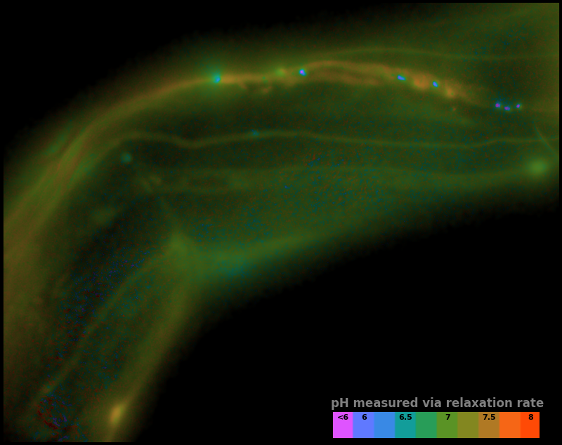
| Measurement type: | ||
| Colormap type: | (see inset colorbar) | |
| Relaxation interval: | (seconds; the amount of time between activation and measurement) |
Colormap type: Hue indicates pH selected, the image luminance shows the density of sensor. Regions with no sensor appear black.
Inset boxes on lower right:
Colorbar; each box shows how a given pH will appear in the image's colormap.
Controls:
With Measurement type: Sensor relaxation rate selected, the "relaxation ratio" is used to infer pH. With Measurement type: Sensor activation rate selected, the "activation nonlinearity" is used to infer pH.
We define the "relaxation ratio" as a pixelwise ratio of differences:
Where '\(\text{Image after deactivation}\)', '\(\text{Image after activation}\)', and '\(\text{Image after relaxation}\)' correspond to frames 1, 10, and 11 of Figure 6, respectively. The relaxation ratio is a simple, robust estimator. As illustrated in Figure 3, it depends strongly on the rate of relaxation, but not on the quantity of sensor or quantity of background, and it depends only weakly on the amount of illumination. By comparing the observed relaxation ratio to a calibration dataset, we can account for the effects of illumination intensity, and convert our map of relaxation ratios to the map of pH vs. position shown in Figure 7.
It's inherently futile to validate a sensor via an in vivo measurement, but the pH map in Figure 7 has several reassuring features. The inferred pH values are broadly consistent with the range we expect in living creatures. Continuous structures have smoothly-varying pH values, suggesting our measured values are not dominated by noise. Distinct structures have distinct pH values, suggesting our measured values are not independent of the sample. Some of the bright punctate structures have especially low pH, but some also have fairly high pH, suggesting our results are not simply an aggregation artifact. While these observations prove nothing, we find them highly encouraging, and consistent with all our experience using pH-Countdown.
In our current implementation, there's a tradeoff between speed and signal-to-noise ratio (SNR). Figure 7 shows measured pH maps for three different values of Relaxation Interval, and the longest interval shows superior SNR compared to the shortest interval. In this case, waiting longer improves SNR, but this is only because our sample holds still.
Opaque creatures
Encouraged by our results in C. elegans, we decided to attempt relaxation sensing in a much more challenging context: living mice. Figure 8 shows pH-Countdown measurements in a live (but anaesthetized) Mus musculus.
| Comparison: |
BAM15 is a "mitochondrial uncoupler" [Kenwood 2014], which has been explored as a potential anti-obesity drug [Alexopoulos 2020]. Mitochondrial uncouplers transport protons into the mitochondrial matrix, which we would expect to lower the mitochondrial pH. By expressing pH-Countdown in the mitochondria of a tumor in a living mouse, we can directly quantitatively interrogate the proposed mechanism of action of this drug.
As shown in Figure 8, the signal from fully subcutaneous mito-pH-Countdown clearly reveals a drug-induced shift in mitochondrial pH, of roughly 0.2 pH units. This agrees qualitatively with similar measurements in cultured cells, where mitochondrial uncouplers rapidly lower mitochondrial pH. However, it disagrees quantitatively with our results when the same cell type is given the same drug in a dish, which yields a shift closer to 1 pH unit. It's not surprising that an animal buffers the effects of a drug on its cells, but it's exciting that we can now measure the difference quantitatively. Note that we can also explore pharmacokinetics; for example, the mitochondrial pH begins to return to baseline in an interval consistent with BAM15's reported half-life (Figure 8 with Comparison: Before and 40 minutes after BAM15).
The mouse is an extremely challenging context for this type of quantitative measurement. In cultured cells, we can use spatial resolution to assign signal to a particular organelle. In the mouse, scattering degrades our spatial resolution by orders of magnitude, and we rely exclusively on genetic targeting for organelle- and tissue-specific measurement. In transparent creatures like the worm, we could measure via either activation or relaxation rates. In the mouse, opacity makes calibrating our illumination intensity effectively impossible, and we can only make quantitative measurements via relaxation rates. In transparent creatures, we can take measurements more rapidly by using homogenous violet illumination to force pH-Countdown into a standard initial condition. In the mouse, opacity prevents deep penetration of violet light, and we must wait for thermal equilibrium if we want to start a measurement in a well-defined steady-state. The paralyzed worm held extremely still, but the heartbeat, breathing, and wiggling of the anaesthetized mouse required image registration to prevent measurement artifacts.
The comparison between in cellulo and in vivo measurements is striking: ~fivefold smaller pH changes, terrible spatial resolution, inhomogenous opacity, and a moving sample. We expect these to be general features of most noninvasive measurements of nonlethal perturbations in vivo, which emphasizes the importance of sensitive, quantitative, robust sensing. Despite these challenges, we were pleased with the repeatability of our measurements; note that each color curve in the right panel of Figure 8 is actually two curves, from two consecutive repetitions of the same measurement. We were pleasantly surprised that this approach worked so well on our first try; we expected mousework to be more frustrating. Of course, if we want to draw meaningful conclusions about BAM15 or mouse physiology, we would repeat this measurement in more mice, and more conditions. Since our primary goal is to establish that this type of optical measurement is possible in principle, we feel n=1 is still useful. To our knowledge, there is currently no other way to take this type of measurement.
Discussion
Will this work in mice that aren't asleep?
One of our ambitions is to enable scientists and researchers to quickly, accurately measure the (sub)cutaneous concentration of a wide range of small molecules in freely-moving animals. We are optimistic, because a dead chicken is roughly optically equivalent to a live chicken. Of course, the dead chicken tends to hold still; to extend relaxation sensing to a wider range of creatures in a wider range of conditions, we need strategies to deal with their motion.
The simple algorithms that produce Figures 5, 6, and 7 use pixelwise subtraction, which assumes the fluorophores at each pixel hold still during relaxation. More generally, we can compare any two regions across time if we're confident the two regions contain the same set of fluorophores. For example, mitochondria move substantially during relaxation, but we can still accurately calculate whole-cell relaxation ratios. This approach trades spatial resolution for simplicity and accuracy, but this may be a useful trade in many contexts. We invite our computationally-skilled colleagues to consider attacking this problem in a more sophisticated way.
Another obvious strategy to enable relaxation sensing in rapidly moving samples is to make relaxation faster. A simple but impractical way to accelerate spontaneous relaxation is to raise the pH or the temperature. A more practical, but longer-term approach is to continue to mutate fluorophores like Countdown and pH-Countdown, while screening for rapid relaxation. We've been doing this successfully for years, and we plan to continue doing so. We expect slow but steady progress; nearly every round of mutagenesis we've done has yielded a slightly faster mutant.
Another strategy to deal with sample motion is to take our data more quickly. In this work, we intentionally used only simple microscopy and photography hardware, which we expect many other labs will also have access to. On such hardware, photoactivating pH-Countdown typically takes at least a few seconds, and relaxation several more. However, with brighter illumination on a faster microscope
[Millett-Sikking 2019],
we can take whole-cell 3D pH-Countdown photoactivation curves in 10-100 ms. As shown in Figures 1, 2, 3 and 6, the activation rate of a relaxation sensor also depends on our quantity of interest, and as shown in Figure 7 with Measurement type: Sensor activation rate, we can use this rate to infer pH. Unfortunately, activation rates also depend on illumination intensity (Figure 3, bottom left panel with Animated quantity: Illumination), but this suggests an approach that uses photoactivation rates for high-speed measurement in transparent creatures, calibrated in situ by slow but accurate relaxation rate measurements.
We note two practical but important details that may ultimately limit the speed of relaxation sensing. While playing with a high-speed camera, we were quite surprised to notice that the autofluorescence of meat (e.g. chicken skin) shows slight photoswitching, with rapid spontaneous recovery on a ~50 ms timescale. This fast dynamic has no impact on our current (slow) approach, but if we succeed in engineering a 10-100x faster relaxation sensor, we'll have to account for this effect. In a similar spirit, we suspect that protonation equilibration times are effectively instantaneous compared to our current slow approach, but may become an important factor in the future.
Finally, we note that relaxation sensing naturally integrates over a finite time window. This is unsuitable for quick measurements in wiggly samples, but we could imagine contexts where measuring a time-averaged quantity is useful. As noted in our Results section, we have a series of mutants with spontaneous decay rates spanning the range from seconds to hours, which could be used to engineer time-integrating sensors.
Can we trust our measurement?
We've done our best to validate pH-Countdown as a reliable sensor, but real validation comes over time from use, experience and community consensus. We have a few suspicions where potential complications may emerge:
- Any sensor which binds a small molecule, even transiently, can affect the effective concentration of that molecule. We suspect that pH-Countdown acts as a "photosponge" for protons, and during rapid photoswitching at high pH-Countdown concentration, could perhaps transiently perturb pH.
- pH-Countdown is a (distant) descendent of Padron, which has a strongly oligomerization-dependent contrast ratio. The relaxation rate of pH-Countdown doesn't seem to depend on concentration in our hands, but presumably there exists some concentration at which oligomerization effects become important.
- We failed to observe substantial off-target sensing, but we emphasize that such testing is never exhaustive.
Does this work for anything but pH?
One of our ambitions is to extend relaxation sensing to a wide range of target molecules (and other quantities of interest). A typical approach to couple a molecule's concentration to a fluorophore is to fuse a naturally-evolved binding domain to a fluorescent protein, as shown in Figure 1 with Binding domain: External to fluorescent domain. The diversity of evolved binding domains provides a straightforward (albeit laborious) path to modularity
[Nakai 2001,
Hung 2011,
Tantama 2013,
Kiyonaka 2013,
van der Linden 2021].
As shown in Figure 1 with Binding domain: Internal to fluorescent domain, pH-Countdown's 'binding domain' for protons is the fluorophore itself; can we demonstrate relaxation sensing with an external domain?
We decided to start with calcium, to build on the substantial labor our peers have already invested in developing and optimizing calcium sensors. We replaced the cpGFP fluorescent domain of the GECO 1.2 sensor [Zhao 2011] with (normal, nonpermuted) pH-Countdown, and screened a variety of linkers for Ca2+-dependent relaxation. As shown in Figure 9, this seems to work!
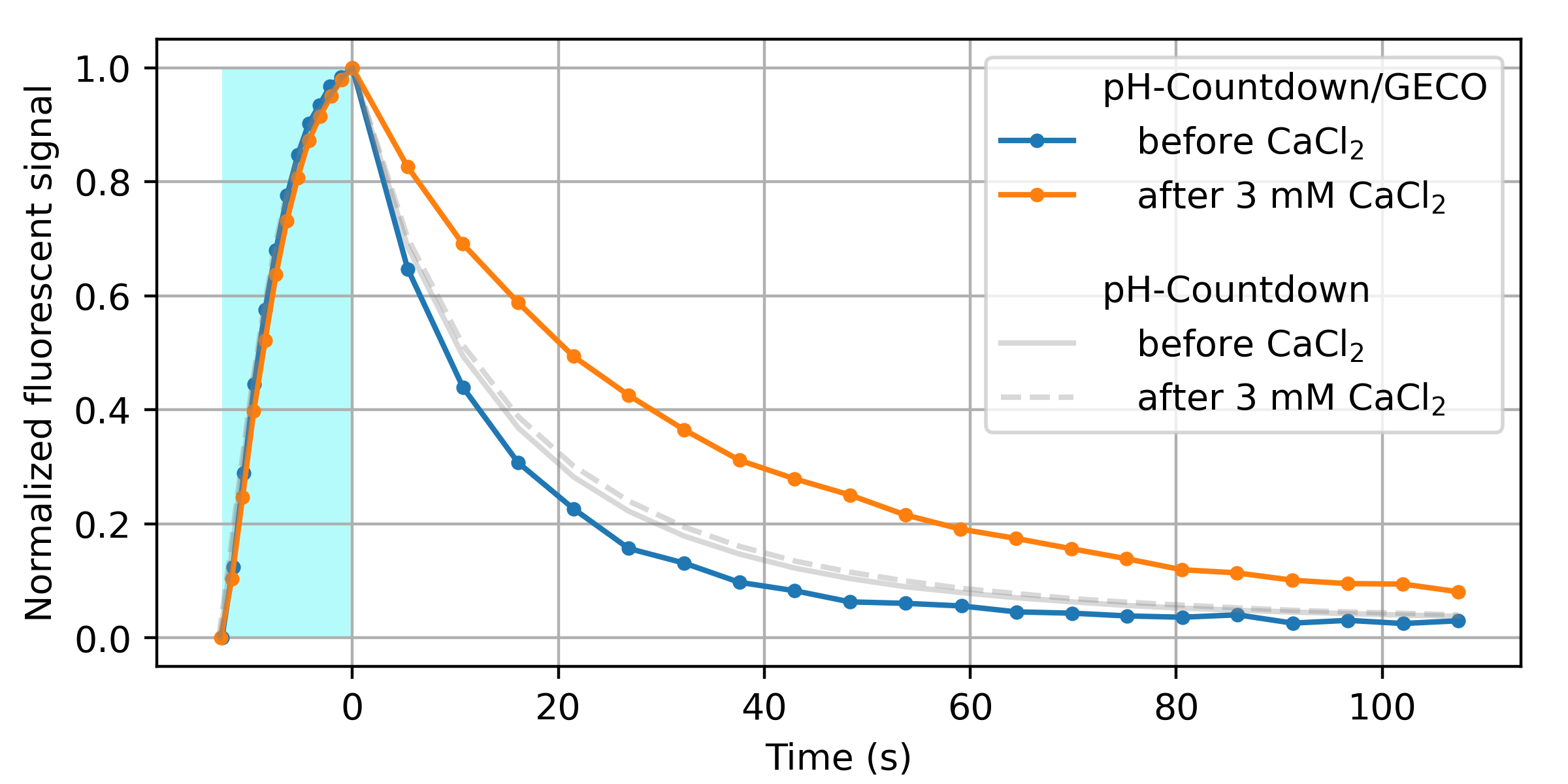
We emphasize that this is just a proof of principle. Before we'd call this a "sensor", we'd prefer to do several rounds of optimization, and extensive validation and characterization. However, we're quite pleased that it seems straightforward to couple a relaxation-based readout to an existing optimized exogenous binding domain. Note that the pH-Countdown fluorescent domain in this fusion is not circularly permuted. We speculate that this is why most of the linkers we screened yielded fluorescent, photoswitching fusions; only the calcium sensitivity seemed to depend on the linker. This makes us cautiously optimisitic about the modularity of relaxation sensing via Countdown, pH-Countdown, and other fluorophores which "relax". We also speculate that if "tugging on the linkers" of a fluorescent protein modifies the relaxation rate, readout via relaxation could report any quantity which can be coupled to "tugging" (e.g. tension).
Does this work for any other fluorophores?
One of our ambitions is to extend relaxation sensing to a wide range of spectral channels. Countdown and pH-Countdown both use the GFP channel; sensors in other colors would allow multiplexing. Red-shifted sensors would be especially useful to improve depth penetration for in vivo measurements. The diversity of engineered fluorescent proteins and molecules provides a huge set of possibilities. Can we identify existing fluorescent domains which "relax", and couple this relaxation rate to a quantity of interest?
A wide variety of GFP-derived fluorophores (e.g. eCFP, eYFP, Citrine) have been observed to spontaneously recover after (apparently) photobleaching during imaging [Sinnecker 2005]. From our perspective, reversible photobleaching followed by spontaneous recovery-in-the-dark is equivalent to photoswitching followed by relaxation. Therefore, we examined an existing cpVenus-based NAD+ biosensor for NAD+-dependent relaxation. As shown in Figure 10, this seems to work!
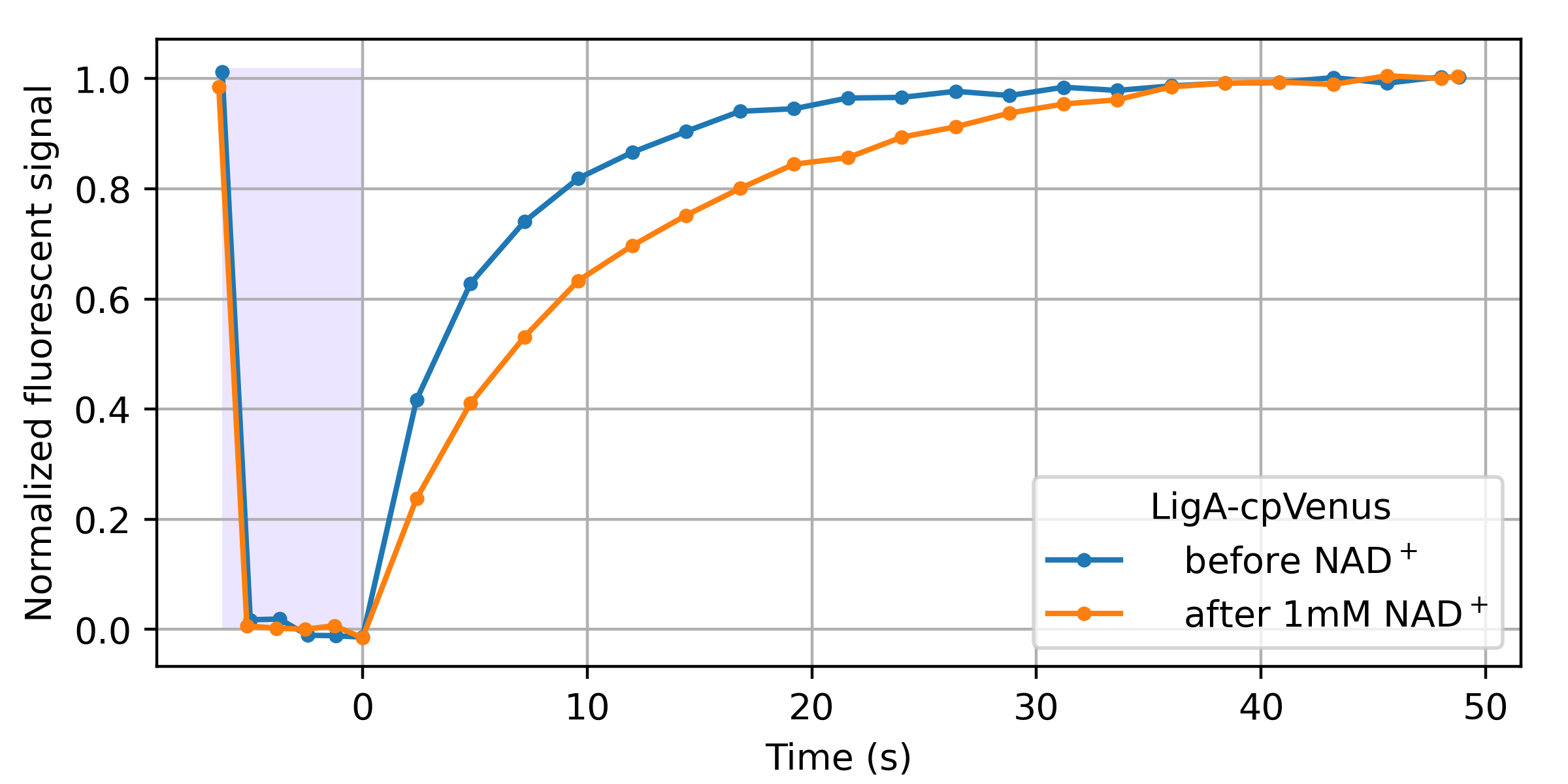
LigA-cpVenus sensing of NAD+ was initially demonstrated via dual-color intensity-ratio-based readout from the single cpVenus fluorescent domain [Cambronne 2016]. As we describe in our introduction, a dual-color intensity ratio can yield simple and accurate sensor readout in transparent, background-free samples. We speculate that since relaxation also depends here on NAD+, relaxation sensing could enable accurate readout in partially opaque, autofluorescent samples. We also suspect that further engineering could enhance this modest, accidental relaxation-based readout to more useful levels. Perhaps other existing sensors are also accidentaly relaxation sensors, and checking for this property could prove useful.
Many other fluorescent proteins have been observed to rapidly "relax", including Dronpa-2, mApple, rsCherryRev, and ShyRFP, and they represent promising alternative starting points for engineering relaxation sensors [Ando 2007, Shaner 2008, Stiel 2008, Shen 2014]. Rhodopsin-based spontaneous switching has also been described as a readout mechanism for fluorescent biosensing [Hou 2014]. Even dyes which spontaneously blink [Uno 2014] could potentially be coupled to quantities of interest [Deo 2021], and read out via relaxation to improve performance in opaque, high-background samples.
Open-source software
As always, our work here depends critically on the open-source software community. Among our crucial dependencies:
- Python
- Numpy [Harris 2020]
- Scipy [Virtanen 2020]
- Matplotlib [Hunter 2007]
- pySerial
- tifffile
- ImageJ [Schneider 2012]
- Micro-Manager [Edelstein 2010]
- FFmpeg
We sincerely thank the authors of these projects for enabling our work.